finally found the meaning of ‘I Like it on the Floor, I like it on my desk..I like it anywhere’ Facebook updates

Ok. I'll just go direct to the point. Read this article http://thenewsoftoday.com/about-the-i-like-it-on-the-floor-i-like-it-anywhere-facebook-status-updates/3239/

October is Breast cancer month and women posting these updates want to show their support. That's it.

lessons from drinking sessions part 2..

Second round of drinking session, this time with my good friend wert, we talked to our friends dad and he shared with us several key points. Below are the things that I remember :).

Key thing that I remember is "never be complacent, strive for greatness and avoid the trap of mediocrity".
Other things he also mentioned are the following:

1. too much analysis leads to paralysis - deal with problems, don't think and analyze too much.
2. marijuana is good. smells good - hehe.. :)
3. be frank, use your position, directly say what you want.
4. experience life, everything is a dose of experience.
5. make mistakes while young...
6. when talking to a crowd, start from where you came from - your foundation and branch your ideas from it. In this way, you are confident that you know what you're talking.

7. In correspondence to number 6, you must establish a solid foundation. whatever that maybe..
8.

..there are still couple of things. I just don't remember, :) hehe

lessons from drinking sessions..part 1.

Nakausap ko si Fidel Rillo habang ako ay nakipag-inuman sa bahay ng aming kaibigan (tawagin natin Mambo) bilang despidida nya papuntang Germany. Nais kong ibahagi ang mga bagay na napagusapan namin.

Tinanong ako ng "What is God?"

• napakahirap na tanong, isang tanong na kahit alam mong iba ang nagtanong sayo ay isa iyong tanong sa sarili mo. Bilang hindi ko alam kung ano ang tamang sagot, sinagot ko na lang ay..uhh, hindi ko pa pinagiisipan yan. hehe
• Isang sagot ang binigay sa akin ng tatay ng aking kaibigan. "it is the search for truth"
• Ako ay isang estudyante ng agham, at kung gagamitan mo ng rason, mahirap mapatunayan kung ano ang tamang sagot. "its the search for truth" -- sa gantong paraan, maaring pagdugtungin ang dalawang bagay na tila magkasalungat.
• It is the search for truth..science and God...

 isa itong palaisipan sa akin, isang bagay na dapat kong sagutin...

abangan ang iba pang mga lessons from drinking sessions :)

Simple way to fight Dengue

I got this email from my colleague and it is worth trying. I recommend doing this at home and provide feedback if it will work.

I don't know where this came from but below is an exact copy of the email. Thank you to whoever made this. I haven't proven its worth but it should be worth a try.. here it goes...

Its just a mix of water, brown sugar and yeast.

1.  Cut a plastic bottle in half, keep both parts. Can be soft drink bottle. 
2. Take the lower portion of the bottle. Dissolve the brown sugar in hot water. Let it cool down to ~70 deg F.
3. Add the yeast. Carbon dioxide will form (This will attract the mosquitoes)
4. Cover the bottle with a dark wrap and  insert in the top portion upside down like a funnel. Place it in a corner in your house. 
5. In 2 weeks you will be surprised by the number of mosquitoes killed.    

 

So there you go. It sounds simple and I hope through this it will help some families out there who are in danger of mosquito diseases..

Activity 19: Restoration of blurred image

In the previous activity, we only considered adding noise but without the application of the degradation function. In this activity, we perform restoration for an image degraded by a known function h(x,y) and added with noise n(x,y) (see FIG 1 of activity 18 for the image degradation and restoration model).

FIG 1: Degradation process of an image f(x,y) by convolution of the degradation function h(x,y) with the image f(x,y) and addition of nosie n(x,y). By the convolution theorem this is represented as multiplication in the frequency domain represented in Eq (2) where capital letters denote the Fourier transform of the smaller letters in Eq (1). The '*' operator denotes convolution.

In this activity we consider uniform linear motion blur and obtain an estimate of the analytical form of this kind of blurring. Thus, we find the transfer function H(u,v) of the motion blur.

Estimate of the degradation function, h
Assuming that the opening and closing of the shutter of the imaging device occurs simultaneously and considering perfect optical imaging process, the degraded image g(x,y) in the frequency domain can be represented by Eq. (2) where the transfer function H follows the form below.

FIG 2: Estimate of the transfer function for uniform linear motion assuming perfect optical imaging and instantaneous opening and closing of the shutter of the imaging device. Where T is the duration of the exposure, a and b are the total distance for which the image was displaced in the x and y direction respectively.

Restoration of the degraded image g(x,y) to f^(x.y)
In this activity, we use the Wiener filter which minimizes the mean square error between the restored image (f^) and the original image f. i.e., min{|f^-f|} The Wiener filter assumes that the image and noise are random processes and ncorporates the statistical properties of the noise and degradation function in the restoration process. The minimum of the mean square error is given below in the frequency domain as:

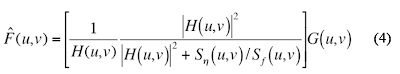FIG 3: Wiener filter. H(u,v) is the degradation function from Eq. (3), |H(u,v)| = H*(u,v)H(u,v) where H*(u,v) above denotes complex conjugation, Sn(u,v) = |N(u,v)|^2 and Sf(u,v) = |F(u,v)| ^2 are the power spectrum of the noise and the undergraded image.

FIG 4: Transfer function H (frequency space, left) and the equivalent function h in real space, (right) for T=1, and a=b=0.01.

The image below shows the results for an image degraded by H and added with a Gaussian noise of mean = 0.01 and var = 0.01 generated using scilab's grand function.

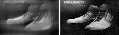FIG 5: Test image degraded by H following the form of Eq. (3) with T=1, a=0.01, b=0.01 and added by a Gaussian noise of mean=0.01 and variance = 0.01. The restoration using Wiener filter of Eq. (4) is visually successful.

Usually when we are dealing with real images, the power spectrum Sf(u,v) of the undergraded image is unknown. We can estimate Eq. (4) by assuming a white noise with a constant power spectrum reducing Eq. (4) to the equation below.

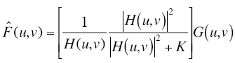FIG 6: Estimate of the Wiener filter.

For different values of K, we reconstruct the degraded image as shown in the images below.

FIG 7: Reconstruction for varying values of K = [1e-4 1e-3 1e-2 1e-1 1] for degraded image with T=1, a=b=0.01 added with Gaussian noise of mean = 0.01 and variance=0.01.

Comparing the Wiener filter reconstruction with the 'estimate of the wiener filter' , the Wiener filter yields better reconstruction as compared to the 'estimate wiener filter'. The reconstruction for the 'estimate of the wiener filter' has good quality when the value of K is close to zero.

For other combinations of a, b and T, the following reconstruction results.

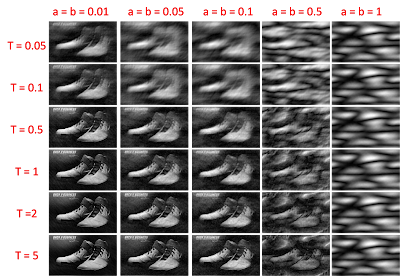FIG 8. Reconstruction for different combinations of T and a=b. Generally, increasing T increases the quality of the image while increasing a=b decreases the quality of the image.

From the above image, increase in T leads to better reconstruction. This result is most logical since increasing the exposure time of the imaging device increases the number of photons detected and thus better image quality. Since a and b indicates the amount that the image is displaced, increasing a and b will lead to further blurring leading to poor image quality.

In this activity, I would give myself a grade of 9 for not knowing if the result is correct. I have doubts with the appearance of my transfer function and from the picture of the blurred image, it does not appear to be resembling that of a uniform linear blur. Instead, blurring seems to occur in both the x,y directions as oppose to single direction. The image cannot possibly move in both axis simultaneously. It is recommended that the form of the transfer function be checked for future research.

Acknowledgements
I would like to acknowledge Mark Jayson Villangca, Luis Buno and Miguel Sison for useful discussions.

References:
[1] Applied Physics 186 Activity 19 manual.

[2] image source

Activity 18: Noise model and basic image restoration

In image restoration, the objective is to recover the original image f(x,y) from the observed image g(x,y) with an a priori knowledge of the degradation process h(x,y) and the noise n(x,y) added on the image. This kind of modeling is shown in the figure below.

FIG 1: Image degradation and restoration model. The original image f(x,y) undergoes degradation by a known process h(x,y) and added with noise n(x,y) leading th the observed image g(x,y). With the use of restoration filters, image restoration aims to recover f(x,y). [1]

In this activity, we only cover half of the image restoration modelling by adding a known noise n(x,y) to the image and performing restoration algorithm to recover the original image. The strength and properties of the noise n(x,y) can be characterized from its probability distribution function PDF shown below for different noise models.

FIG 2: PDF of the different noise models used characterized by its mean and variance. (click to zoom)

The different noise models were generated using scilab's builtin grand and imnoise function. The Rayleigh noise was generated using a module modnum downloaded from [2] while the other noise were generated using grand and imnoise (see scilabs documentation for more detail on these functions). Below is the resulting image after adding different noise to a test image.

FIG 3: Image histograms after addition of different noise models.

Restoring in the presence of noise

Below are the different noise-reduction filters used when only noise is added to the image [1].

FIG 4: Mean filtering methods for a window of size m x n.

Consider a window, i.e., 3x3 window, we perform the 'mean filtering' on this window. For each pixel in the noisy image g(x,y), we choose a window and perform mean filtering for that pixel. This was done for all the pixels in the images. In order for the algorithm to be effective around the boundaries, the image was tiled in the manner below:

FIG 5: Tiled image to wrap the boundary conditions. The red window represents the area where the spatial noise filtering was applied.

The following pictures below show the result of the restoration process using the different mean filtering methods in FIG 4 for each noise model. The window used is 5x5 and the restoration for the contraharmoic was divided into two depending on the value of Q, {Q=2 & Q=-2}.

FIG 6: Image restoration results for an image added with a Gaussian noise. Looking at the histogram, the restoration was generally successful for all methods except for some error on the shift of the graylevel value of the three peaks in the original image. In particular, geometric, harmonic and contra-harmonic (Q=-2) appear to shift the graylevel value to the right (towards white) relative to arithmetic and contra-harmonic (Q=2). This means that the image shifted to the left will appear darker relative to those shifted to the right.

FIG 7: Image restoration results for an image added with a Rayleigh noise. The restoration of the arithmetic and geometric filtering appears visually correct while for the contra-harmonic filtering, the image is either shifted to the left (Q=2) or right (Q=-2) depending on the value of Q used. Unlike geometric and arithmetic filtering, the histogram of harmonic and contra-harmonic filtering is wider along the peaks of the original image.

FIG 8: Image restoration results for an image added with a Gamma noise. In general, the restoration appears successful except for the contraharmoic (Q=2) restoration where the histogram of the image is more wider.

FIG 9: Image restoration results for an image added with an exponential noise. The contraharmonic restoration (Q=2 & Q=-2) failed in restoring the image due to wide histogram and overshifting to the left of the grayvalues. This degree of shifting is also manifested in the harmonic filtering.

FIG 10: Image restoration results for an image added with a uniform noise. In general, the restoration is quite successful for all methods.

FIG 11: Image restoration results for an image added with a salt & pepper noise. The restoration seems to have artifacts - presence of extra graylevel values. This could be attributed to the strength of the noise used which might be too strong and filtering on a 5 x 5 window is not sufficient to recover the image.

FIG 12. Applying the restoration process to a grayscale image shown above obtained from my brothers collection of images.

Applying this restoration to a grayscale image (obtained from my brother's picture collection), we perform the same method, adding a known noise term to the image and restoring the image using the mean filters of FIG 4.

FIG 13: Grayscale image added with Gaussian noise with the corresponding restorations.

FIG 14: Grayscale image added with Rayleigh noise with the corresponding restorations.

FIG 15: Grayscale image added with Gamma noise with the corresponding restorations.

FIG 16: Grayscale image added with an exponential noise with the corresponding restorations.

FIG 17: Grayscale image added with a uniform noise with the corresponding restorations.

FIG 18: Grayscale image added with salt & pepper noise with the corresponding restorations.

In general, geometric and arithemetic filtering work for all kinds of noise models presented. In particular, the author recommends geometric mean as it seems to be flexible and suitable enough for all noise models studied above.

In this activity, I give myself a grade of 10 for performing the restoration and doing all the required activities.

Acknowledgement

I would like to acknowledge Gilbert Gubatan for providing the downloaded modnum module for generating Rayleigh noise and my brother for lending one of his collection pictures.

References
[1] Image Restoration. fromhttp://www.ph.tn.tudelft.nl/~lucas/education/et2720in/2002/ImageRestoration.pdf
[2] http://www.scicos.org/ScicosModNum/modnum_web/src/modnum_421/interf/scicoslab/help/eng/htm/rayleigh_sim.htm

Activity 17: Photometric Stereo

Photometric stereo is a technique that extracts surface elevation by computing the surface normals assuming the intensity is directly proportional to brightness. Using N light sources (V) , the surface normal of each point in the image can be computed following the steps in the image below. (click to zoom for clearer picture)

applying these steps to four light sources with images below, we reconstruct the corresponding shape elevation.

The result is shown below:

The reconstruction is relatively correct but with 'horns' on top and on the edges. Also the image is not smooth and some filtering is recommended.

In this activity, I give myself a grade of 10 for successfully reconstructing the image.

I would like to thank Martin Tensuan for useful discussions.

References:
[1] Applied Physisc 187 Manual (c)2008 Maricor Soriano