In the previous activity, we only considered adding noise but without the application of the degradation function. In this activity, we perform restoration for an image degraded by a known function h(x,y) and added with noise n(x,y) (see FIG 1 of activity 18 for the image degradation and restoration model).

FIG 1: Degradation process of an image f(x,y) by convolution of the degradation function h(x,y) with the image f(x,y) and addition of nosie n(x,y). By the convolution theorem this is represented as multiplication in the frequency domain represented in Eq (2) where capital letters denote the Fourier transform of the smaller letters in Eq (1). The '*' operator denotes convolution.
In this activity we consider uniform linear motion blur and obtain an estimate of the analytical form of this kind of blurring. Thus, we find the transfer function H(u,v) of the motion blur.
In this activity we consider uniform linear motion blur and obtain an estimate of the analytical form of this kind of blurring. Thus, we find the transfer function H(u,v) of the motion blur.
Estimate of the degradation function, h
Assuming that the opening and closing of the shutter of the imaging device occurs simultaneously and considering perfect optical imaging process, the degraded image g(x,y) in the frequency domain can be represented by Eq. (2) where the transfer function H follows the form below.

FIG 2: Estimate of the transfer function for uniform linear motion assuming perfect optical imaging and instantaneous opening and closing of the shutter of the imaging device. Where T is the duration of the exposure, a and b are the total distance for which the image was displaced in the x and y direction respectively.
Restoration of the degraded image g(x,y) to f^(x.y)
In this activity, we use the Wiener filter which minimizes the mean square error between the restored image (f^) and the original image f. i.e., min{|f^-f|} The Wiener filter assumes that the image and noise are random processes and ncorporates the statistical properties of the noise and degradation function in the restoration process. The minimum of the mean square error is given below in the frequency domain as:
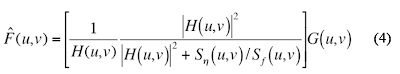 FIG 3: Wiener filter. H(u,v) is the degradation function from Eq. (3), |H(u,v)| = H*(u,v)H(u,v) where H*(u,v) above denotes complex conjugation, Sn(u,v) = |N(u,v)|^2 and Sf(u,v) = |F(u,v)| ^2 are the power spectrum of the noise and the undergraded image.
 FIG 4: Transfer function H (frequency space, left) and the equivalent function h in real space, (right) for T=1, and a=b=0.01.
The image below shows the results for an image degraded by H and added with a Gaussian noise of mean = 0.01 and var = 0.01 generated using scilab's grand function.
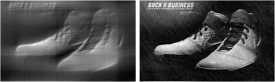 FIG 5: Test image degraded by H following the form of Eq. (3) with T=1, a=0.01, b=0.01 and added by a Gaussian noise of mean=0.01 and variance = 0.01. The restoration using Wiener filter of Eq. (4) is visually successful.
Usually when we are dealing with real images, the power spectrum Sf(u,v) of the undergraded image is unknown. We can estimate Eq. (4) by assuming a white noise with a constant power spectrum reducing Eq. (4) to the equation below.
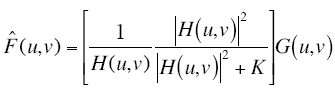 FIG 6: Estimate of the Wiener filter.
 FIG 7: Reconstruction for varying values of K = [1e-4 1e-3 1e-2 1e-1 1] for degraded image with T=1, a=b=0.01 added with Gaussian noise of mean = 0.01 and variance=0.01.
Comparing the Wiener filter reconstruction with the 'estimate of the wiener filter' , the Wiener filter yields better reconstruction as compared to the 'estimate wiener filter'. The reconstruction for the 'estimate of the wiener filter' has good quality when the value of K is close to zero.
For other combinations of a, b and T, the following reconstruction results.
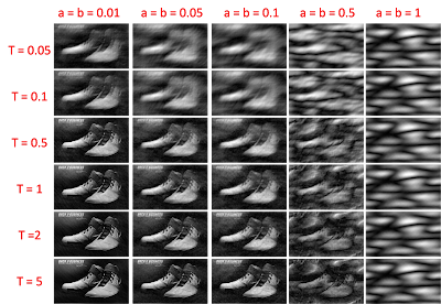 FIG 8. Reconstruction for different combinations of T and a=b. Generally, increasing T increases the quality of the image while increasing a=b decreases the quality of the image.
From the above image, increase in T leads to better reconstruction. This result is most logical since increasing the exposure time of the imaging device increases the number of photons detected and thus better image quality. Since a and b indicates the amount that the image is displaced, increasing a and b will lead to further blurring leading to poor image quality.
In this activity, I would give myself a grade of 9 for not knowing if the result is correct. I have doubts with the appearance of my transfer function and from the picture of the blurred image, it does not appear to be resembling that of a uniform linear blur. Instead, blurring seems to occur in both the x,y directions as oppose to single direction. The image cannot possibly move in both axis simultaneously. It is recommended that the form of the transfer function be checked for future research.
Acknowledgements
I would like to acknowledge Mark Jayson Villangca, Luis Buno and Miguel Sison for useful discussions.
References:
[1] Applied Physics 186 Activity 19 manual.
Restoration of the degraded image g(x,y) to f^(x.y)
In this activity, we use the Wiener filter which minimizes the mean square error between the restored image (f^) and the original image f. i.e., min{|f^-f|} The Wiener filter assumes that the image and noise are random processes and ncorporates the statistical properties of the noise and degradation function in the restoration process. The minimum of the mean square error is given below in the frequency domain as:
 FIG 3: Wiener filter. H(u,v) is the degradation function from Eq. (3), |H(u,v)| = H*(u,v)H(u,v) where H*(u,v) above denotes complex conjugation, Sn(u,v) = |N(u,v)|^2 and Sf(u,v) = |F(u,v)| ^2 are the power spectrum of the noise and the undergraded image.
 FIG 4: Transfer function H (frequency space, left) and the equivalent function h in real space, (right) for T=1, and a=b=0.01.
The image below shows the results for an image degraded by H and added with a Gaussian noise of mean = 0.01 and var = 0.01 generated using scilab's grand function.
 FIG 5: Test image degraded by H following the form of Eq. (3) with T=1, a=0.01, b=0.01 and added by a Gaussian noise of mean=0.01 and variance = 0.01. The restoration using Wiener filter of Eq. (4) is visually successful.
 FIG 6: Estimate of the Wiener filter.
For different values of K, we reconstruct the degraded image as shown in the images below.

Comparing the Wiener filter reconstruction with the 'estimate of the wiener filter' , the Wiener filter yields better reconstruction as compared to the 'estimate wiener filter'. The reconstruction for the 'estimate of the wiener filter' has good quality when the value of K is close to zero.
For other combinations of a, b and T, the following reconstruction results.
 FIG 8. Reconstruction for different combinations of T and a=b. Generally, increasing T increases the quality of the image while increasing a=b decreases the quality of the image.
From the above image, increase in T leads to better reconstruction. This result is most logical since increasing the exposure time of the imaging device increases the number of photons detected and thus better image quality. Since a and b indicates the amount that the image is displaced, increasing a and b will lead to further blurring leading to poor image quality.
In this activity, I would give myself a grade of 9 for not knowing if the result is correct. I have doubts with the appearance of my transfer function and from the picture of the blurred image, it does not appear to be resembling that of a uniform linear blur. Instead, blurring seems to occur in both the x,y directions as oppose to single direction. The image cannot possibly move in both axis simultaneously. It is recommended that the form of the transfer function be checked for future research.
Acknowledgements
I would like to acknowledge Mark Jayson Villangca, Luis Buno and Miguel Sison for useful discussions.
References:
[1] Applied Physics 186 Activity 19 manual.