Activity 3: Image types and basic image enhancement

Digitize image comes in four different types. They are,

• Binary image which are either 1 or 0, black or white. For an image of size 128 x 128 pixels, each pixel occupies 1 bit, so 128 x 128 = 2048bytes or 2KB.
• Grayscale image which contain 8 bits of information. That is, their pixel value can span the range between 0-255. Since it contains 8 bits of information, each pixel occupies 1 byte, for an image of 128x128 pixels = 16384 bytes or 16KB.
• Truecolor image is equivalent to 3 grayscale images called channels. Truecolor images are also know as RGB because each R, G, B represent the 3 different channels of the image (red, green and blue). Per pixel, there are 256^3 possible combination of information. Most colored photos, i.e, taken using digital cameras are RGB.
• Indexed images are color images that contain index numbers mapped to a color map. Thus, they contain two data, the colormap and image. They are generally smaller in file size compared to RGB but less color information because the maximum colors it can contain are indicated in the colormap.

Below are examples of different types of images.
JPEG images of Lena obtained from this source [1]. Note of the difference in file size between the different image file types: Truecolor (RgB), grayscale and binary (black and white).











File Properties: RGB (72.4KB) Grayscale (26KB) Black and white (5KB) Index(31.6KB)
*(http://www.ee.columbia.edu/~cylin/course/mss/MSS_hw1.html)

In the next part, we are going to apply what we learned in activity 2 by obtaining the area of a scanned image. I would like to acknowledge Mark Jayson 'master' Villangca for lending me his scanned image for this activity. In order to check if our area calculation is correct, a ruler was placed side by side with the image. We can then obtain a pixel:physical unit calibration to obtain the true area of the image.

FileName: master.png

FileSize: 208681
Format: PNG
Width: 905
Height: 446
Depth: 8
StorageType: truecolor
NumberOfColors: 0
ResolutionUnit: centimeter
XResolution: 59.050000
YResolution: 59.050000

In order to obtain the area of the image above, we need to binarize the image using im2bw. In doing this, we need to select the correct threshold using the histogram of the image.
Histogram of the above image using my own code for histogram below,
function histogram = fhistogram(img, depth)
bits=(2^depth)-1;
histogram = zeros(bits,2);
bins = 0.5:bits; bins = bins./bits; //bins for [0,1] image.
for i=1:bits,
frequency(i) = sum(img>=(bins(i)-1/(2*bits))&img<(bins(i)+1/(2*bits))); end; histogram(:,1)=bins'; histogram(:,2)=frequency; endfunction

From the histogram we can choose a suitable threshold (i.e, ~ pixel value of 100). Using im2bw, we can then set the threshold (since 0-1, divide 100 by 255) and specify the ROI in the image by defining another matrix. In the above image, we opted to remove the ruler in the thresholding and focused on the image.

Resulting image after converting to binary and applying a region of interest
After using the contour follow, we obtain the contour of the image.

Using the algorithm in activity 2, we obtain the following results
Area of master = 16576 pixels.
Pixel count = 16894 pixels.
Observe the converted binary image has extra white pixels outside the contour 'master'.

In order to calibrate this to physical units we can obtain the pixel:physical ratio using paint. (i.e., we obtained 1cm:30pixels ~ ). Thus the area of the contour in physical units is
Area = 552.533 cm^2.

For this activity I give myself a grade of 9 for finishing the activity although a bit late and additional bonus for providing my own code for the histogram.

I would like to acknowledge Mark Jayson Villangca for lending me the scanned image. Jica and Miguel for useful discussions.

References:
[1] Activity 3 manual.

[2] http://www.ee.columbia.edu/~cylin/course/mss/MSS_hw1.html

Activity 2: Area Estimation of Images with Defined Edges

Area estimation finds many applications in the field of material science, biology, geology and the natural science in general . Biologists are especially interested in the difference in size between cancer cells and healthy cells. In material science, area measurement of leads and semiconductor materials among others is an effective tool for processing and failure analysis. In geology, remote sensing is an active area of research used widely in environmental and marine science researches [1].

The method below discusses image area measurement using Green's Theorem. It must be noted that before using this method, there are several limitations that must be considered. We will discuss these limitations at the end of the article.

We start with the following.
Below are sample images (256 x 256 ) of triangle, square, circle and several irregular polygons which we will use in our area estimation method.

Circle of diameter=125px, Square of side=130px, triangle of base=height=150px. These measurements are obtained from MS Paint while creating the images. It must be noted that these measurements are just guidelines for checking our results and must not be used as the theoretical area of the image. In creating these images, the border already occupied several pixels, so the area of the shape (white) does not necessarily reflect the analytically expected result. (i.e, Area_square = 130*130)

Pixel Count: 16129
Computed Area: 16129

Pixel Count: 11644
Computed Area: 11644


Pixel Count: 10731
Computed Area: 10731

Pixel Count: 17522
Computed Area: 17522

Pixel Count: 14058
Computed Area: 14056

Pixel Count: 14913
Computed Area: 7414

In order to compute the area of the above images, we use the SIP toolbox of scilab-4.1.2 using the command follow. Excerpt from the description of follow command from scilab:

"follow - A contour follower. Function follow extracts parametric contours of binary objects. This is useful for further extracting object features such as curvature and bending energy."

Note that before we use the command follow, our images must be first binarize. This can be done in scilab using the command im2bw. The command follow returns the [x,y] coordinates of the contour. We can then use this contour coordinates to compute the area using Green's Theorem found below. For more detailed discussion of area measurement using Green's Theorem please follow this source [2] (http://www.attewode.com/Calculus/AreaMeasurement/area.htm).

Since the image is binarized, we can compute the thoretical area by summing the pixels of the image (white~1 and black~0). We designated the theoretical area as "pixel count" in the above images and "computed area" when using Green's Theorem.

Below is the code in scilab used to obtain the pixel count and the computed area:

//load image
directory='C:\Documents and Settings\2004-29578\Desktop\Activities\Activity 2\'
filename='quadrilateral_130side.jpg';
img1= imread(directory+filename);

//binarize image
img2=im2bw(img1, 0.5);

//get the contour using follow
[x,y]=follow(img2);
//get the dimensions of x and y
[M,N]=size(x)
//complete the contour setting the last pixel=first pixel
x(M+1)=x(1);
y(M+1)=y(1);

plot(x,y);

//get the area using Greens Theorem. we use round since the area (number of pixels (1 or 0)) can only take //integer values.
Area = round(0.5*sum((x(1:M).*y(2:(M+1)))-(y(1:M).*x(2:(M+1)))))+ round((M+1)/2);
//pixel count
TArea = sum(img2);

//imshow to scale to grascale, i.e., highest pixel becomes white, lowest pixel becomes black
//binarize image using im2bw
//increase memory for scilab use, stacksize.

Note that in obtaining the computed area, we added a correcting factor "round((M+1)/2)" in our code where M is the length of the x or y vector.

Results and Limitations
(1) For the regular polygons and the first irregular polygon, the pixel count and the computed area are the same, meaning that the algorithm successfully estimated the area of the images.
(2) For the next irregular polygon (figure batman) there is a discrepancy in the pixel count and the computed area.

In the figure above, note the extra 2 pixels in 'batman's" horn which accounted for the discrepancy. This error is due to the command "follow" of scilab which assumes only ONE contour per image. In order to check this, we made two contours in the next image and as expected there is a huge discrepancy between the pixel count and the computed area.

(3) The algorithm and theory for computing the area is pretty solid (Green's Theorem) hence most of our errors should come from the input and processing of the input. That is, our limitations will most probably due to the command follow and im2bw of scilab.

Overlayed image of the binared square and its contour using the command follow. Note that there is an offset in the contour compared to the image of ~2 pixels. Similar observation is found in the next image.
Note the offset between the contour and the image.

(4) The command im2bw is similar to thresholding and thus depending on your threshold, the computed area will change. This effect would most probably depend on the user setting the threshold and making measurements.

(5) It is expected that in large scale images (2048x2048) the computed area will approach the analytical area. This would be very useful in applications like remote sensing and geological survey.

For this activity, I give myself a grade of 10 for exact area measurement as proven by the sets of images used.

References:

[1] Activity 2 Handout
[2] http://www.attewode.com/Calculus/AreaMeasurement/area.htm

Activity 1: Digital Scanning

excerpt from activity 1 handout...
"In this activity, we use ratio and proportion to find the numerical values of a digitally scanned hand-drawn plot. For now, you will need the following software, Paint for finding the pixel locations on the graph, and Excel of Open Office Spreadsheet to tabulate the values of the graph."

What I did.
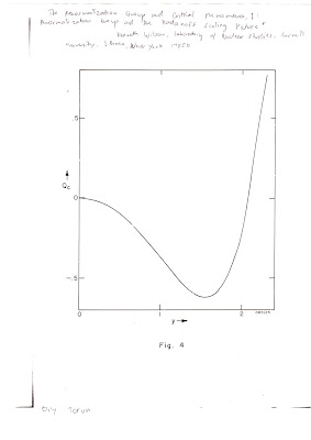
1. Photocopied a plot from the College of Science Libray from the following journal.
The Renormalization Group and Cricitical Phenomena I: Renormalization Group and the Kardanoff Scaling Picture by Kenneth Wilson from the Laboratory of Nuclear Studies, Cornell University, Ithaca New York, 14850 on 1974.

The photocopied image was then digitally scanned. (see picture below)
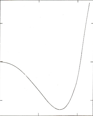
For convenience, I cropped the image at the origin resulting to the image below.
The cropped image was then opened in MS Paint.
Producing the Plot in Open Office:
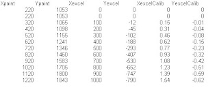
Using MS Paint, the pixel location of the origin was recorded. Note that in paint, the (0,0) mark is at the top-left of the document. In this activity, the pixel location of the origin of the cropped image is at (220,1053).

Using Open Office, I successively obtained the pixel locations of the graph at 50 pixel interval in the x-axis amounting to 33 data points. Using the pixel locations of the origin, I calibrated the pixel location obtained previously by noting that the top-left part of Paint is the (0,0) mark using the following formula:
Xexcel=Xpixel-220,
Yexcel=1053-Ypixel (see picture below for sample data points)


Next, I obtained the number of pixels/unit in the graph and obtained the following:
Pixels/unit in the x-axis = 648
Pixels/unit in the y-axis = 1276
Using this calibration I divided all the values of the Xexcel by 648 and all values of Yexcel by 1276. This will give the calibrated values of the graph in physical units.

In order to check if the reconstructed image and the original image are perfectly matched, the two images were overlayed. This can be easily done in open office by importing the scanned image as graphic. (Format->graphic->bitmap->import the image). After importing the image, click on the reconstructed graph and set the Area to the imported image (click on the graph->object properties->area->select bitmap->select your imported image).

At first, the images will not be perfectly matched. In order to overlay it perfectly, you must obtain the maximum locations of the grid in the x and y axis. Use this and modify the axes of the graph and set it to the obtained maximum.

The image below is the reconstructed image overlayed with the scanned image.
Observe that the image grids in the scanned image and the reconstructed image are perfectly matched. Furthermore, the graph is well-matched with no visible offset. For this activity, I give myself a grade of 10 for perfectly reconstructing the scanned image.