Activity 18: Noise model and basic image restoration

In image restoration, the objective is to recover the original image f(x,y) from the observed image g(x,y) with an a priori knowledge of the degradation process h(x,y) and the noise n(x,y) added on the image. This kind of modeling is shown in the figure below.

FIG 1: Image degradation and restoration model. The original image f(x,y) undergoes degradation by a known process h(x,y) and added with noise n(x,y) leading th the observed image g(x,y). With the use of restoration filters, image restoration aims to recover f(x,y). [1]

In this activity, we only cover half of the image restoration modelling by adding a known noise n(x,y) to the image and performing restoration algorithm to recover the original image. The strength and properties of the noise n(x,y) can be characterized from its probability distribution function PDF shown below for different noise models.

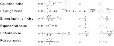
FIG 2: PDF of the different noise models used characterized by its mean and variance. (click to zoom)

The different noise models were generated using scilab's builtin grand and imnoise function. The Rayleigh noise was generated using a module modnum downloaded from [2] while the other noise were generated using grand and imnoise (see scilabs documentation for more detail on these functions). Below is the resulting image after adding different noise to a test image.

FIG 3: Image histograms after addition of different noise models.

Restoring in the presence of noise

Below are the different noise-reduction filters used when only noise is added to the image [1].

FIG 4: Mean filtering methods for a window of size m x n.

Consider a window, i.e., 3x3 window, we perform the 'mean filtering' on this window. For each pixel in the noisy image g(x,y), we choose a window and perform mean filtering for that pixel. This was done for all the pixels in the images. In order for the algorithm to be effective around the boundaries, the image was tiled in the manner below:

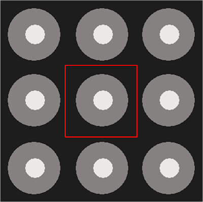
FIG 5: Tiled image to wrap the boundary conditions. The red window represents the area where the spatial noise filtering was applied.

The following pictures below show the result of the restoration process using the different mean filtering methods in FIG 4 for each noise model. The window used is 5x5 and the restoration for the contraharmoic was divided into two depending on the value of Q, {Q=2 & Q=-2}.

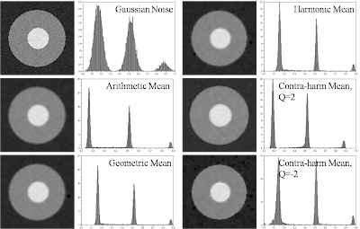FIG 6: Image restoration results for an image added with a Gaussian noise. Looking at the histogram, the restoration was generally successful for all methods except for some error on the shift of the graylevel value of the three peaks in the original image. In particular, geometric, harmonic and contra-harmonic (Q=-2) appear to shift the graylevel value to the right (towards white) relative to arithmetic and contra-harmonic (Q=2). This means that the image shifted to the left will appear darker relative to those shifted to the right.

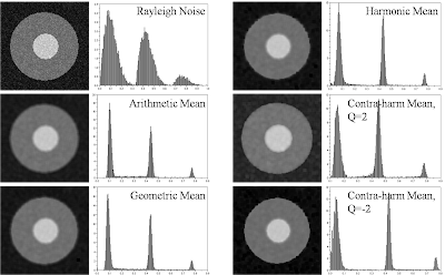FIG 7: Image restoration results for an image added with a Rayleigh noise. The restoration of the arithmetic and geometric filtering appears visually correct while for the contra-harmonic filtering, the image is either shifted to the left (Q=2) or right (Q=-2) depending on the value of Q used. Unlike geometric and arithmetic filtering, the histogram of harmonic and contra-harmonic filtering is wider along the peaks of the original image.

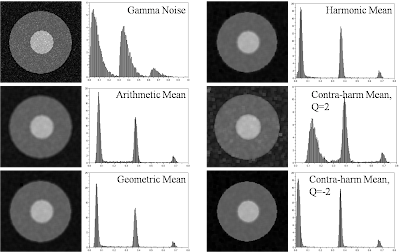FIG 8: Image restoration results for an image added with a Gamma noise. In general, the restoration appears successful except for the contraharmoic (Q=2) restoration where the histogram of the image is more wider.

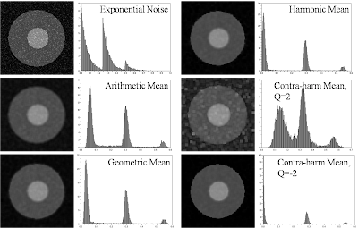FIG 9: Image restoration results for an image added with an exponential noise. The contraharmonic restoration (Q=2 & Q=-2) failed in restoring the image due to wide histogram and overshifting to the left of the grayvalues. This degree of shifting is also manifested in the harmonic filtering.

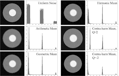FIG 10: Image restoration results for an image added with a uniform noise. In general, the restoration is quite successful for all methods.

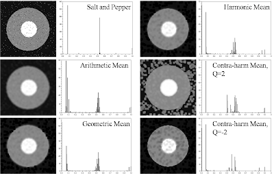FIG 11: Image restoration results for an image added with a salt & pepper noise. The restoration seems to have artifacts - presence of extra graylevel values. This could be attributed to the strength of the noise used which might be too strong and filtering on a 5 x 5 window is not sufficient to recover the image.

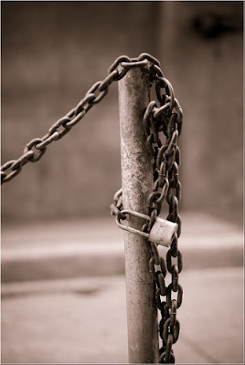FIG 12. Applying the restoration process to a grayscale image shown above obtained from my brothers collection of images.

Applying this restoration to a grayscale image (obtained from my brother's picture collection), we perform the same method, adding a known noise term to the image and restoring the image using the mean filters of FIG 4.

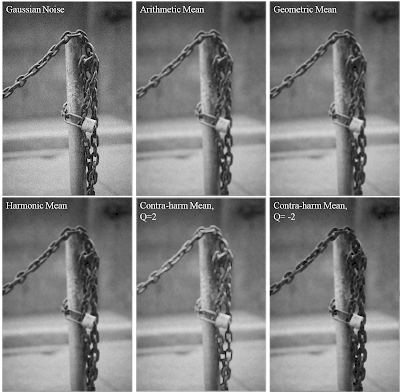
FIG 13: Grayscale image added with Gaussian noise with the corresponding restorations.

FIG 14: Grayscale image added with Rayleigh noise with the corresponding restorations.

FIG 15: Grayscale image added with Gamma noise with the corresponding restorations.

FIG 16: Grayscale image added with an exponential noise with the corresponding restorations.

FIG 17: Grayscale image added with a uniform noise with the corresponding restorations.

FIG 18: Grayscale image added with salt & pepper noise with the corresponding restorations.

In general, geometric and arithemetic filtering work for all kinds of noise models presented. In particular, the author recommends geometric mean as it seems to be flexible and suitable enough for all noise models studied above.

In this activity, I give myself a grade of 10 for performing the restoration and doing all the required activities.

Acknowledgement

I would like to acknowledge Gilbert Gubatan for providing the downloaded modnum module for generating Rayleigh noise and my brother for lending one of his collection pictures.

References
[1] Image Restoration. fromhttp://www.ph.tn.tudelft.nl/~lucas/education/et2720in/2002/ImageRestoration.pdf
[2] http://www.scicos.org/ScicosModNum/modnum_web/src/modnum_421/interf/scicoslab/help/eng/htm/rayleigh_sim.htm